Stippling and TSP art in R: emulating StippleGen

Stippling is the creation of a pattern simulating varying degrees of solidity or shading by using small dots (Wikipedia).StippleGen is a piece of software that renders images using stipple patterns, which I discovered on Xi’an’s blog a couple days ago.

Stippled version of a sketch by Paul Cézanne, rendered in R


Read more…

Superpixels in imager

Superpixels are used in image segmentation as a pre-processing step. Instead of segmenting pixels directly, we first group similar pixels into “super-pixels”, which can then be processed further (and more cheaply).


(image from Wikimedia)

The current version of imager doesn’t implement them, but it turns out that SLIC superpixels are particularly easy to implement. SLIC is essentially k-means applied to pixels, with some bells and whistles.

Read more…

New version of imager package for image processing

A new version of imager is now available on CRAN. This release brings a lot of new features, including a whole new set of functions dealing with pixel sets, better support for videos, new and faster reduction functions.

The most significant change is the introduction of a “pixset” class, which deals with sets of pixels (for instance, the set of all pixels with a certain brightness, the foreground, the left-hand side of an image, an ROI, etc.). The pixset class includes many tools for working with pixsets, described in a new vignette.

Read more…

vecpack: an R package for packing stuff into vectors

Here’s a problem I’ve had again and again: let’s say you’ve defined a statistical model with several parameters. One of them is a scalar. Another is a matrix. The third one is a vector, and so on. When fitting the model the natural thing to do is to write a likelihood function that takes as many arguments as you have parameters in your model: i.e., lik(x,y,z) where x is a scalar, y a matrix and z a vector. The problem is that, while it’s the natural way of writing that function, that’s not what optimisers like “optim” want: they want a function with a single argument, and that argument should be a vector. So you have to pack everything into a vector, and write a whole lot of boilerplate code to unpack all the parameters out of that vector.

vecpack saves you from having to write all that boilerplate:


devtools::install_github("dahtah/vecpack")

library(vecpack)

#A cost function in two arguments:
cost <- function(a,b)  (3*a-b+2)^2

#Call optim via vpoptim
res <- vpoptim(list(a=1,b=0),cost)
res$par

vecpack knows how to automatically pack and unpack scalars, vectors, matrices and images (from the imager package). It’s also very easy to extend.

The package is quite new, and not on CRAN yet. Feedback welcome, either here or on the issues page on github.


New features in imager 0.30

imager is an R package for image processing, based on CImg. This new release brings many new features, including:

  • Support for automatic parallel processing using OpenMP.
  • A new S3 class, imlist, which makes it easy to work with image lists
  • New functions for interactively selecting image regions (grabRect,grabPoint,grabLine)
  • Experimental support for CImg’s byte-compiled DSL via imeval, patch_summary.
  • Improved plotting, API consistency, and documentation

To get started with imager, see the tutorial. Some of the new features are detailed below the fold.

And now, for your viewing pleasure, the following piece of code downloads a random cat picture, and makes a video of a bouncing kitten:

library(rvest)
library(imager)
#Run a search query (returning html content)
search <- read_html("https://www.google.com/search?site=&tbm=isch&q=cat")
#Grab all <img> tags, get their "src" attribute, a URL to an image
urls <- search %>% html_nodes("img") %>% html_attr("src") #Get urls of parrot pictures

#Load the first image, and resize 
sprite <- load.image(urls[1]) %>% resize(150,150)

#We'll use 30 frames
t <- seq(0,1,l=30)

#Equations of motion
xt <- function(t) 250*t
yt <- function(t) 400- 1100*abs(t-.5)
alpha <- function(t) 1-1.8*abs(t-.5)

#An empty frame for our cat
im <- imfill(400,400,val=rep(0,3))

#Let's make our video
vid <- lapply(t,function(t) imdraw(im,sprite,x=xt(t),y=yt(t),opacity=alpha(t))) %>% imappend("z")

play(vid,loop=TRUE,normalise=FALSE)

output

Read more…

New features in imager 0.20

imager, an R package for image processing, has been updated to v0.20 on CRAN. It’s a major upgrade with a lot of new features, better documentation and a more consistent API.

imager now has 130 functions, and I myself keep forgetting all that’s in there. I’ve added a tutorial vignette that should help you get started. It goes through a few basic tasks like plotting and histogram equalisation and builds up to a multi-scale blob detector. It also covers plotting with ggplot2 and has a thematic list of functions.

blobs

New features added in the last months include new assignment functions, a utility for getting information on image files (iminfo), auto-thresholding based on k-means, much better array subset operators, updated docs and a reorganised codebase. Windows support should also have improved. Last but not least, you can now interrupt lengthy computations by hitting Ctrl+c or the stop button in RStudio.

imager now has some easy-to-use replacement functions, meaning you can now do set image channels or change frames using a convenient R-like syntax:

library(imager)
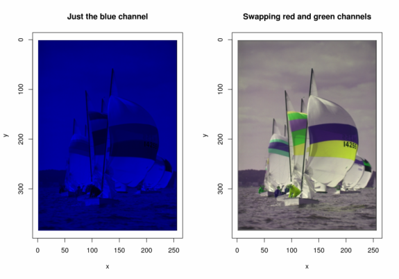
boats.cp = boats #Make a copy of the boats image
R(boats.cp) = 0 #Set red channel to 0
G(boats.cp) =  0 #Set blue channel to 0
plot(boats.cp,main="Just the blue channel")
R(boats.cp) = G(boats)
G(boats.cp) = R(boats)
plot(boats.cp,main="Swapping red and green channels")

ab
see ?imager.replace for more.

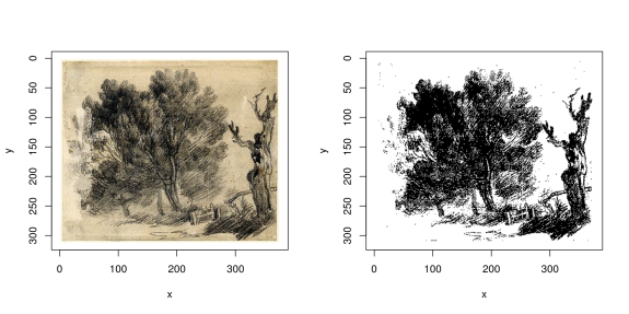
Auto-thresholding finds an optimal threshold for converting an image to binary values, based on k-means (it’s essentially a variant of Otsu’s method).
Here’s an illustration on a sketch by Thomas Gainsborough:

url = "https://upload.wikimedia.org/wikipedia/commons/thumb/3/30/Study_of_willows_by_Thomas_Gainsborough.jpg/375px-Study_of_willows_by_Thomas_Gainsborough.jpg"
im <- load.image(url)
layout(t(1:2))
plot(im)
grayscale(im) %>% threshold %>% plot

unnamed-chunk-2-1

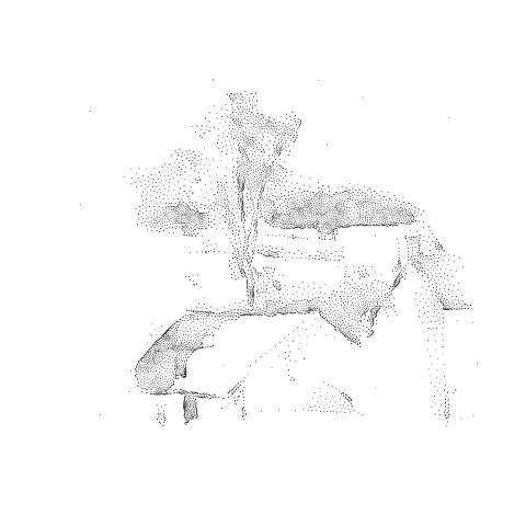
Point-wise reductions are useful for combining a list of images into a single output image. For example, enorm(list(A,B,C)) computes  \sqrt{A^2+B^2+C^2} , ie. the Euclidean norm. Here’s how you can use it to compute gradient magnitude:

imgradient(im,"xy") %>% enorm %>% plot("Gradient magnitude")

unnamed-chunk-3-1

See also parmax, parmin, add, etc .

A note on compiling imager: if for some reason R tries to install imager from source (Linux or Mac), you will need the fftw library. On a Mac the easiest way is to grab it via Homebrew (“brew install fftw”), in Ubuntu “sudo apt-get install libfftw3-dev” should do it.

New R package for Eyelink eye-trackers

Eyelink eye-trackers output an avalanche of disorganised crap. I’ve written an R package that will hopefully filter that crap for you. It’s called eyelinker and it’s on Github.

It outputs a set of dataframes containing raw traces, saccades, fixations and blinks, meaning it’s easy to produce plots like this one:

example_eyelinker

There’s a vignette explaining everything, just hit vignette(“basics”,package=”eyelinker”).

I’ve tested it on some of our local datasets but given the relatively free-form nature of Eyelink asc files, there’s no guarantee it will work everywhere.

Bug reports are welcome on the github issues page.

imager now on CRAN, and a non-linear filtering example

imager is an R package for image processing that’s fairly fast and now quite powerful (if I may say so myself). It wraps a neat C++ library called CImg, by David Tschumperlé (CNRS). It took quite a bit of work, but imager is now on CRAN, so that installing it is as easy as:

install.packages("imager")

Here’s an example of using imager for max-filtering. A max-filter replaces each pixel value with the maximum value of its neighbours. Usually you’d write a loop, but we want to do things the R way (warning: this only works for small neighbourhoods, for reasons that will become obvious).

library(imager)
im <- load.image(system.file('extdata/parrots.png',package='imager'))
nhood <- expand.grid(dx=-2:2,dy=-2:2) #We want to include all pixels in a square 5x5 neighbourhood
im.s <- alply(nhood,1,function(d) imshift(im,d$dx,d$dy))

The result is a list of shifted versions of the image im (there are 5×5 = 25 different shifts, so you can imagine that you wouldn’t want to do this with a 20×20 neighbourhood and a large image!)
Now running a max (or min) filter is just a matter of calling pmax (or pmin):

max.filt <- do.call(pmax,im.s)
min.filt <- do.call(pmin,im.s)

Here’s our max-filtered image:

maxfilt

and here’s the min-filtered one:

minfilt

New package for image processing in R

[update: imager is now on CRAN. install via install.packages(“imager”)]

I’ve written a package for image processing in R, with the goal of providing a fast API in R that lets you do things in C++ if you need to. The package is called imager, and it’ on Github.
The whole thing is based on CImg, a very nice C++ library for image processing by David Tschumperlé.

Features:

  • Handles images in up to 4 dimensions, meaning you can use it for volumetric/hyperspectral/data or short videos
  • Facilities for taking subsets of images, pixel neighbourhoods, etc.
  • All the usual image processing stuff (filters, morphology, transformations, interpolation, etc.)
  • Easy access to the C++ API via Rcpp

The package is still in an early phase but it can already do a lot of useful things as you’ll see from the documentation.

Example code:

library(imager)
im <- load.image(system.file('extdata/parrots.png',package='imager'))
layout(t(1:3)) 
plot(im,main="Original image")
grad <- grayscale(im) %>% get_gradient("xy")
names(grad) <- paste("Gradient along",c("x","y")) 
l_ply(names(grad),function(n) plot(grad[[n]],main=n))

example_parrots

Visit the website for more information.

Neurostats 2014 Highlights

Last week the Neurostats 2014 workshop took place at the University of Warwick (co-organised by Adam Johansen, Nicolas Chopin, and myself). The goal was to put some neuroscientists and statisticians together to talk about neural data and what to do with it. General impressions:

  • The type of Bayesian hierarchical modelling that Andrew Gelman has been advocating for years is starting to see some use in neuroimaging. On the one hand it makes plenty of sense since the data at the level of individual subjects can be cr*p and so one could really use a bit of clever pooling. On the other, imaging data is very high-dimensional, running a Gibbs sampler can take days, and it’s not easy making the data comparable across subjects.
  • You have to know your signals. Neural data can be unbelievably complicated and details matter a lot, as Jonathan Victor showed in his talk. A consequence if that if you as a neuroscientist have a data analysis problem, it’s not enough to go see a statistician and ask for advice. If you have EEG data you need to find someone who knows *specifically* about all the traps and pitfalls of EEG, or else someone who’s willing to learn about these things. A consequence is that we should think about training neurostatisticians, the way we already have biostatisticians, econometricians and psychometricians.

There were plenty of interesting talks, but below are some of my personal highlights.

Read more…